Annotate XCMS peaklist
Jan Stanstrup
2023-11-03
from_peaklist.RmdThis tutorial contains references to specific chromatograhic systems in use at NEXS, University of Copenhagen and might be confusing to others.
If you want a copy of this Rmarkdown tutorial you can do the following, which will create a copy in your working folder:
file.copy(system.file("doc/from_peaklist.Rmd", package="XCMSAnnotator"), ".")If you would rather have a script you can do:
knitr::purl(system.file("doc/from_peaklist.Rmd", package="XCMSAnnotator"))Load some required packages
library(tidyverse)
library(XCMSAnnotator)
library(MetaboAnnotation)
library(ProtGenerics)
library(conflicted)
conflicts_prefer(dplyr::filter)
conflicts_prefer(MetaboAnnotation::matches)
If you are missing packages you can run
devtools::install_gitlab("stanstrup_r_packages/xcms-annotator").
Loading your peaklist
Our first objective is to take a peaklist and convert it to spectra.
Spectra is a special object type that holds MS spectra. We
do the conversion based on annotation from CAMERA and we
assume each pcgroup can be considered a spectrum.
We load an example peaklist that has been converted to long format. In long format every row represents 1 peak found in 1 sample.
peaklist_long <- read_csv("https://nexs-metabolomics.gitlab.io/INM/inm-booklet/peaklist_long.csv")

peaklist_long
## # A tibble: 49,590 × 59
## ...1 mode feature_id D_ratio f_mzmed f_mzmin f_mzmax f_rtmed f_rtmin
## <dbl> <chr> <dbl> <dbl> <dbl> <dbl> <dbl> <dbl> <dbl>
## 1 1 NEG 1 0.0541 81.0 81.0 81.0 167. 164.
## 2 2 NEG 1 0.0541 81.0 81.0 81.0 167. 164.
## 3 3 NEG 1 0.0541 81.0 81.0 81.0 167. 164.
## 4 4 NEG 1 0.0541 81.0 81.0 81.0 167. 164.
## 5 5 NEG 1 0.0541 81.0 81.0 81.0 167. 164.
## 6 6 NEG 1 0.0541 81.0 81.0 81.0 167. 164.
## 7 7 NEG 1 0.0541 81.0 81.0 81.0 167. 164.
## 8 8 NEG 1 0.0541 81.0 81.0 81.0 167. 164.
## 9 9 NEG 1 0.0541 81.0 81.0 81.0 167. 164.
## 10 10 NEG 1 0.0541 81.0 81.0 81.0 167. 164.
## # ℹ 49,580 more rows
## # ℹ 50 more variables: f_rtmax <dbl>, isotopes <chr>, adduct <chr>,
## # pcgroup <dbl>, ms_level <dbl>, filepath <chr>, filename <chr>, desc <chr>,
## # msfile <chr>, inletfile <chr>, bottle <chr>, injection_vol <dbl>,
## # sample_type <chr>, MSE <lgl>, inj_order <dbl>, subject <dbl>, time <dbl>,
## # gender <chr>, drink <chr>, fromFile <dbl>, peakidx <dbl>, mz <dbl>,
## # mzmin <dbl>, mzmax <dbl>, rt <dbl>, rtmin <dbl>, rtmax <dbl>, into <dbl>, …For the following workflow the peaklist should adhere to the following rules:
- it should have at least the following columns:
filename,feature_id,into,f_mzmed,f_rtmed,pcgroup,ionmode,project. - the column
ionmodeis expected to have the ionization mode defined by being either"pos"or"neg".
In this example the project column doesn’t exist, so we
create a dummy column that is always "dummy". The mode
column in this example has the wrong capitalization (apart from also
being mode instead of ionmode) so we make a
new column ionmode where that is fixed.
We can now convert the peaklist to a Spectra object (the
last function, peaklist_to_spectra does that).
peaklist_spectra_joined <- peaklist_long %>%
                            mutate(project = "dummy") %>% # make a dummy column that says "dummy"
                            mutate(ionmode = if_else(mode == "POS", "pos", "neg")) %>% # new column with correct specification
                            peaklist_to_spectra() # do the conversion to spectra.

peaklist_spectra_joined
## MSn data (Spectra) with 586 spectra in a MsBackendMemory backend:
## msLevel rtime scanIndex
## <integer> <numeric> <integer>
## 1 NA 204.452 NA
## 2 NA 167.047 NA
## 3 NA 183.655 NA
## 4 NA 130.676 NA
## 5 NA 151.804 NA
## ... ... ... ...
## 582 NA 32.4068 NA
## 583 NA 206.9142 NA
## 584 NA 26.2725 NA
## 585 NA 202.9672 NA
## 586 NA 28.8145 NA
## ... 19 more variables/columns.
## Processing:
## Merge 586 Spectra into one [Mon Oct 27 15:10:49 2025]You can see that msLevel and scanIndex are NA. That is
fine. We don’t need them.
Read database
Now we read your database of compounds that was created by MScurate and filter it for a specific machine.
DB <- readRDS(system.file("extdata/DB.rds", package="XCMSAnnotator"))

DB_selected <- DB %>%
                spectraData %>%
                as_tibble %>%
                pull(dataOrigin) %>%
                grep("Qtof", .) %>% # We want only the standards that have "Qtof" in the path.
                {DB[.]}


DB_selected
## MSn data (Spectra) with 958 spectra in a MsBackendDataFrame backend:
## msLevel rtime scanIndex
## <integer> <numeric> <integer>
## 1 1 421.556 1606
## 2 1 311.221 1186
## 3 1 288.769 1099
## 4 1 421.047 1608
## 5 1 410.298 1564
## ... ... ... ...
## 954 1 174.107 663
## 955 1 46.407 176
## 956 1 357.088 1361
## 957 1 317.121 NA
## 958 1 297.348 1131
## ... 48 more variables/columns.
## Processing:
## Merge 2304 Spectra into one [Mon Sep 27 13:09:49 2021]Project RT of database to the system that was used for the peaklist
The standards we selected above were run on our Premier Q-tof machine (It also contains data from the Synapt). But the chromatograhic method is our so-called “Quat” method, while the data from the peaklist was generated using the so called “new method”.
For this reason the retention times won’t match between the database and the peaklist. We can however fix that by using PredRet, that is able to project the RTs from one system to another.
We first load all the PredRet projection models:
predret_models <- readRDS(system.file("extdata/predret_models.rds", package="XCMSAnnotator"))We can then check which systems are available (there won’t be models between all possible pairs!):
predret_list_systems(predret_models)## [1] "A1"
## [2] "ABC"
## [3] "Acquity HSST3 - RP - 60 mn"
## [4] "ACQUITY UPLC HSS C18 QTOF 20min"
## [5] "AjsTestF"
## [6] "AjsUoB"
## [7] "Bade_Publi"
## [8] "BDD_C18"
## [9] "BfG_NTS_RP1"
## [10] "C18_SOP3"
## [11] "Cao_HILIC"
## [12] "CBM_Test_A"
## [13] "CBM_Test_A_"
## [14] "CBM_Test_B"
## [15] "CBM_Test_C"
## [16] "CBM_Test_D"
## [17] "CBM_Test_E"
## [18] "CBM_TEST_F"
## [19] "CBM_Test_G"
## [20] "cecum_JS"
## [21] "Chen_Waters_SERI2019_58PFAS"
## [22] "CS1"
## [23] "CS10"
## [24] "CS11"
## [25] "CS12"
## [26] "CS13"
## [27] "CS14"
## [28] "CS15"
## [29] "CS16"
## [30] "CS17"
## [31] "CS18"
## [32] "CS19"
## [33] "CS2"
## [34] "CS20"
## [35] "CS21"
## [36] "CS22"
## [37] "CS23"
## [38] "CS24"
## [39] "CS3"
## [40] "CS4"
## [41] "CS5"
## [42] "CS6"
## [43] "CS7"
## [44] "CS8"
## [45] "CS9"
## [46] "Eawag_XBridgeC18"
## [47] "FEM_lipids"
## [48] "FEM_long"
## [49] "FEM_orbitrap_plasma"
## [50] "FEM_orbitrap_urine"
## [51] "FEM_short"
## [52] "HIILIC_tip"
## [53] "HILIC_BDD_2"
## [54] "hypergold_pea"
## [55] "ICPR_Harmon_MeOH_Method_BfG"
## [56] "IJM_TEST"
## [57] "IPB_Halle"
## [58] "JKD_Probiotics"
## [59] "JP_RP"
## [60] "JS"
## [61] "KI_GIAR_zic_HILIC_pH2_7"
## [62] "LIFE_new"
## [63] "LIFE_old"
## [64] "Luca_Hilic_UGR"
## [65] "Luca_RP_UGR"
## [66] "LucaUGR"
## [67] "Mceachran HPLC #1"
## [68] "Meister zic-pHILIC pH9.3"
## [69] "MPI_Symmetry"
## [70] "MTBLS20"
## [71] "MTBLS20-LIUMIN"
## [72] "MTBLS36"
## [73] "MTBLS38"
## [74] "MTBLS39"
## [75] "MTBLS87"
## [76] "MultiConditionRT1112.7"
## [77] "MultiConditionRT11210"
## [78] "MultiConditionRT1132"
## [79] "MultiConditionRT1142"
## [80] "MultiConditionRT1155"
## [81] "MultiConditionRT1165"
## [82] "MultiConditionRT1168"
## [83] "MultiConditionRT1178"
## [84] "MultiConditionRT1212.7"
## [85] "MultiConditionRT12210"
## [86] "MultiConditionRT1232"
## [87] "MultiConditionRT1242"
## [88] "MultiConditionRT1255"
## [89] "MultiConditionRT1265"
## [90] "MultiConditionRT1268"
## [91] "MultiConditionRT1278"
## [92] "MultiConditionRT2112.7"
## [93] "MultiConditionRT21210"
## [94] "MultiConditionRT2132.1"
## [95] "MultiConditionRT2142"
## [96] "MultiConditionRT2155"
## [97] "MultiConditionRT2165"
## [98] "MultiConditionRT2168"
## [99] "MultiConditionRT2178"
## [100] "MultiConditionRT2212.7"
## [101] "MultiConditionRT22210"
## [102] "MultiConditionRT2232"
## [103] "MultiConditionRT2242"
## [104] "MultiConditionRT2255"
## [105] "MultiConditionRT2265"
## [106] "MultiConditionRT2268"
## [107] "MultiConditionRT2278"
## [108] "MultiConditionRT3112.7"
## [109] "MultiConditionRT3113"
## [110] "MultiConditionRT3115"
## [111] "MultiConditionRT3143"
## [112] "MultiConditionRT3145"
## [113] "MultiConditionRT3212"
## [114] "MultiConditionRT3213"
## [115] "MultiConditionRT3215"
## [116] "MultiConditionRT3243"
## [117] "MultiConditionRT3245"
## [118] "MultiConditionRT4112.7"
## [119] "MultiConditionRT4212.7"
## [120] "NEXS-prem-met-quat"
## [121] "NEXS-syn-met-new"
## [122] "OBSF"
## [123] "PFR-TK72"
## [124] "qqq_myco"
## [125] "re"
## [126] "RIKEN"
## [127] "RPFDAMM"
## [128] "RPLC_zorbax150_JH"
## [129] "RPMMFDA"
## [130] "RWS_QE_IKSR_MECN"
## [131] "RWS_QE_IKSR_MEOH"
## [132] "SMRT"
## [133] "SNU_organoid"
## [134] "SNU_RIKEN_POS"
## [135] "SNU_RP_10"
## [136] "SNU_RP_108"
## [137] "SNU_RP_20"
## [138] "SNU_RP_30"
## [139] "SNU_RP_50"
## [140] "SNU_RP_70"
## [141] "SNU_RP_indole_annotation"
## [142] "SNU_RP_indole_order"
## [143] "SNU-test"
## [144] "TEST"
## [145] "test_SNU_tip"
## [146] "UFZ_Phenomenex"
## [147] "UniToyama_Atlantis"
## [148] "Waters ACQUITY UPLC with Synapt G1 Q-TOF"
## [149] "Waters STA Forensic"We can see all the possible models like this:
View(predret_list_models(predret_models))## # A tibble: 3,113 × 11
## name_sys1 name_sys2 n_points mean_error_abs median_error_abs q95_error_abs
## <chr> <chr> <int> <dbl> <dbl> <dbl>
## 1 FEM_short CS1 16 0.147 0.108 0.475
## 2 FEM_short CS17 16 1.03 0.478 2.79
## 3 FEM_short CS20 11 0.948 0.536 3.18
## 4 FEM_short CS14 14 0.815 0.286 3.23
## 5 FEM_short CS18 16 0.497 0.383 1.40
## 6 FEM_short CS19 16 0.180 0.186 0.355
## 7 LIFE_new FEM_lipids 10 0.159 0.123 0.353
## 8 LIFE_new CS5 10 0.418 0.148 1.58
## 9 LIFE_new CS14 10 0.315 0.00239 1.64
## 10 LIFE_old Waters ACQU… 10 1.88 1.24 4.03
## # ℹ 3,103 more rows
## # ℹ 5 more variables: max_error_abs <dbl>, mean_ci_width_abs <dbl>,
## # median_ci_width_abs <dbl>, q95_ci_width_abs <dbl>, max_ci_width_abs <dbl>A note on the system at NEXS: Two of the systems appear under two names:
- “LIFE_old” == “CS22”: “old method” run on Qtof
- “LIFE_new” == “CS23”: “new method” run on Qtof
In addition we have the newer methods:
- “NEXS-prem-met-quat”: The “Quat method” run on Qtof Premier
- “NEXS-syn-met-new” : The “new method” run on Synapt
We can now find the model we need to do the projection:
predret_models_selected <- predret_models %>%
                              filter(name_sys1 == "NEXS-prem-met-quat", name_sys2 == "LIFE_new")
And lets plots what the relationship looks like so we can get an idea of how good the model is.
predret_plot_model(predret_models_selected)## Warning in geom_point(data = plotdata_points, aes(rt_from, rt_to, text =
## inchi), : Ignoring unknown aesthetics: text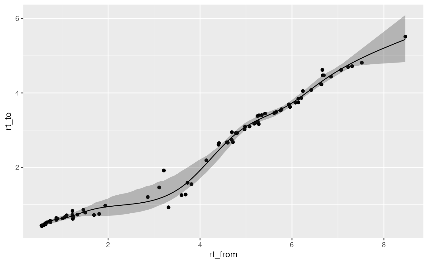
Pretty good model! Notice the confidence interval. That gives an idea of how strict you can be with the RT matching.
Now we can use the model to convert the RTs in the database:
DB_selected_predRT <- predret_project_DB(DB_selected, predret_models_selected, model_rt_multiplier = 60)

DB_selected_predRT
## MSn data (Spectra) with 924 spectra in a MsBackendDataFrame backend:
## msLevel rtime scanIndex
## <integer> <numeric> <integer>
## 1 1 276.833 1606
## 2 1 193.722 1186
## 3 1 175.929 1099
## 4 1 276.459 1608
## 5 1 268.214 1564
## ... ... ... ...
## 920 1 65.4765 663
## 921 1 34.2905 176
## 922 1 221.5842 1361
## 923 1 197.4131 NA
## 924 1 183.5542 1131
## ... 48 more variables/columns.
## Processing:
## Merge 2304 Spectra into one [Mon Sep 27 13:09:49 2021]
## Filter: select retention time [0..Inf] on MS level(s) [Mon Oct 27 15:11:03 2025]It has a few less compounds than before because we cannot extrapolate outside the RT range of the model.
Match database to peaklist
We can now match the DB and the peaklist. First we setup some matching criteria.
mp <- MatchForwardReverseParam(ppm = 30,
                               requirePrecursor = FALSE,
                               THRESHFUN = function(x) which(x > 0),
                               THRESHFUN_REVERSE = function(x) which(x >= 0.7), # so only keep matches if the reverse score is better than 0.7
                               toleranceRt = 0.5*60 # 0.5 min tolerance. Because of the projection we add some margin
                               )
We do the matching:
mtches <- matchSpectra(peaklist_spectra_joined, DB_selected_predRT, param = mp)To avoid splitting both the database and the peaklist we have matching across polarities, which obvious doesn’t make sense. So here we remove matching that are not between spectra of the same polarity.
mtches_mode <- filterMisMatchedPolarity(mtches, query_mode_col = "ionmode", target_mode_col = "polarity")

mtches_mode
## Object of class MatchedSpectra
## Total number of matches: 84
## Number of query objects: 586 (67 matched)
## Number of target objects: 924 (74 matched)The report above tells you how many matches you have.
If you have a peaklist that mixes two projects (like
urine and fecal) you can split them like this:
project_idx1 <- spectraData(query(mtches_mode))$project[mtches_mode@matches$query_idx] == unique(spectraData(mtches_mode)$project)[1]
project_idx2 <- spectraData(query(mtches_mode))$project[mtches_mode@matches$query_idx] == unique(spectraData(mtches_mode)$project)[2]

mtches_mode_pro1 <- filterMatches(mtches_mode,
                                  SelectMatchesParam(
                                    index = which(project_idx1),
                                    keep = TRUE
                                  )
)


mtches_mode_pro2 <- filterMatches(mtches_mode,
                                  SelectMatchesParam(
                                    index = which(project_idx2),
                                    keep = TRUE
                                  )
)
We don’t have that here so we won’t do that.
Write report
Now we can write out a pdf with a nice report of the matches. This can take quite a while. Be patient!
create_annotation_report(
                          mtches_mode,
                          outname = "annotate_report", # without extension!
                          outpath = ".", # means the folder you are in
                          skip_latex_dependency_check = FALSE,
                          title = "Annotation project",
                          author = "Meeeee!"
)
## /usr/bin/pandoc +RTS -K512m -RTS annotate_report.knit.md --to latex --from markdown+autolink_bare_uris+tex_math_single_backslash --output annotate_report.tex --lua-filter /usr/local/lib/R/site-library/rmarkdown/rmarkdown/lua/pagebreak.lua --lua-filter /usr/local/lib/R/site-library/rmarkdown/rmarkdown/lua/latex-div.lua --embed-resources --standalone --highlight-style tango --pdf-engine xelatex --variable graphics --include-in-header /tmp/RtmpUO0zfA/rmarkdown-str1c204e844b44.html## [1] TRUEReport with only matches
We can also get a report with only the matches by setting
only_matches = TRUE.
create_annotation_report(
                          mtches_mode,
                          outname = "annotate_report_only_matches", # without extension!
                          outpath = ".", # means the folder you are in
                          skip_latex_dependency_check = FALSE,
                          title = "Annotation project",
                          author = "Meeeee!",
                          only_matches = TRUE
)
## /usr/bin/pandoc +RTS -K512m -RTS annotate_report.knit.md --to latex --from markdown+autolink_bare_uris+tex_math_single_backslash --output annotate_report.tex --lua-filter /usr/local/lib/R/site-library/rmarkdown/rmarkdown/lua/pagebreak.lua --lua-filter /usr/local/lib/R/site-library/rmarkdown/rmarkdown/lua/latex-div.lua --embed-resources --standalone --highlight-style tango --pdf-engine xelatex --variable graphics --include-in-header /tmp/RtmpUO0zfA/rmarkdown-str1c2060b26b87.html## [1] TRUEFind higest intensity peaks
It is often useful to find the samples with the highest intensity when you want to look at the raw data or plan your MS/MS experiments. So lets find the most intense samples for each feature we have matched to the database.
First we find the relevant pcgroups:
matched_pc_groups <- mtches_mode@query %>%
                        spectraData() %>%
                        as_tibble %>%
                        slice(matches(mtches_mode)$query_idx) %>%
                        distinct(ionmode, pcgroup)

matched_pc_groups
## # A tibble: 67 × 2
## ionmode pcgroup
## <chr> <dbl>
## 1 neg 1
## 2 neg 2
## 3 neg 3
## 4 neg 9
## 5 neg 10
## 6 neg 12
## 7 neg 20
## 8 neg 23
## 9 neg 30
## 10 neg 31
## # ℹ 57 more rowsNext we extract from the peaklist the most intense samples:
peaklist_long2 <- peaklist_long %>% mutate(ionmode = if_else(mode == "POS", "pos", "neg")) # fix the ionmode notation again.

ID_table <- matched_pc_groups %>%
                left_join(peaklist_long2, by = c("ionmode", "pcgroup")) %>%
                distinct(ionmode, feature_id) %>%
                left_join(peaklist_long2, by = c("ionmode", "feature_id")) %>%
                group_by(ionmode, pcgroup, feature_id) %>%
                group_nest() %>%
                mutate(most_intense = map_chr(data, ~ ..1 %>%
                                                arrange(desc(into)) %>%
                                                slice(1:3) %>% # first to third most intense
                                                pull(filename) %>%
                                                paste(collapse=", ")
                                              )
                       ) %>%
                select(ionmode, pcgroup, feature_id, most_intense)

ID_table
## # A tibble: 133 × 4
## ionmode pcgroup feature_id most_intense
## <chr> <dbl> <dbl> <chr>
## 1 neg 1 102 2011-12-06-103.mzML, 2011-12-06-077.mzML, 2011-12…
## 2 neg 1 105 2011-12-06-077.mzML, 2011-12-06-080.mzML, 2011-12…
## 3 neg 1 111 2011-12-06-077.mzML, 2011-12-06-080.mzML, 2011-12…
## 4 neg 1 399 2011-12-06-077.mzML, 2011-12-06-080.mzML, 2011-12…
## 5 neg 2 1 2011-12-06-077.mzML, 2011-12-06-080.mzML, 2011-12…
## 6 neg 2 148 2011-12-06-077.mzML, 2011-12-06-080.mzML, 2011-12…
## 7 neg 2 149 2011-12-06-077.mzML, 2011-12-06-093.mzML, 2011-12…
## 8 neg 2 285 2011-12-06-077.mzML, 2011-12-06-091.mzML, 2011-12…
## 9 neg 2 416 2011-12-06-077.mzML, 2011-12-06-080.mzML, 2011-12…
## 10 neg 2 482 2011-12-06-091.mzML, 2011-12-06-103.mzML, 2011-12…
## # ℹ 123 more rows